Introduction to Variational Auto-Encoders

ML Researcher
In my previous post, I went through what an Autoencoder is, how it works, and how to build and apply it to the (toy) MNIST dataset. As a refresher, an Auto-Encoder is a type of neural network that attempts to copy its inputs into its outputs via a hidden layer which describes code or latent factors. The encoder codifies input data into this latent space, and the decoder attempts to reconstruct the original input data given some sort of constraint depending on the use case.
In this post, I take this further with the concept of the Variational Autoencoder, first introduced by Diederik Kingma and Max welling in their 2013 paper, Auto-Encoding Variational Bayes
Modeling Data
Let's assume we have data which are generated from a random process, using an unobserved continuous random variable z. Not to over-complicate this with unnecessary math: $$p(\text{x}|\textbf{z})p(\textbf{z})$$
Breaking down the above, the right term is a hidden, unobserved process parameterized by \(\theta\), our prior distribution. The left hand side is a process conditioned on this prior, and the entire term is proportional to our posterior distribution.
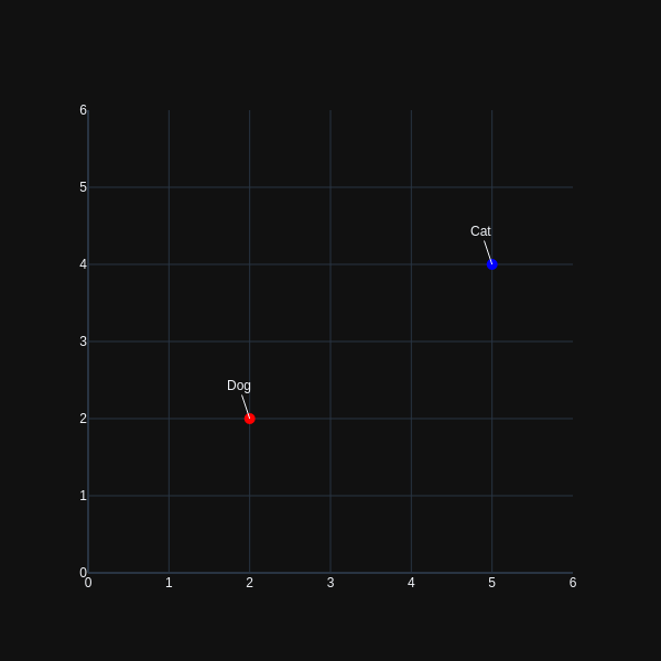
For a more concrete example, let's assume we are attempting to encode pictures of cats and dogs using our auto-encoder. For your non-probabilistic, conventional auto-encoder, the cat and dog classes may be encoded as single points in latent space. If, for the sake of example, latent-space exists in two dimensions, our cat and dog class might be represented in a manner similar to that as shown below.
Now if the decoder part of our encoder attempts to reconstruct the original data from the encoding above, the chance for choosing a 'valid' point in latent space to re-generate input images is significantly less. If instead, the probabilistic encoder encodes our input data using a continuous distribution(in two-dimensional space):
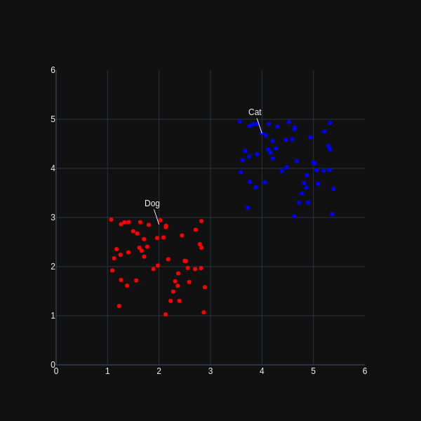
the chance of selecting a 'valid' point is significantly higher, in addition to providing valid variations derived from the original input data. The other, less obvious advantage is that a distribution of points more effectively models the inherent uncertainty in the encoder's approximation of the original input data.
Variational Auto-Encoder
The VAE was proposed to address two main issues which arise when attempting to model the distribution of data:
- The case when the true posterior density and the integral of the marginal likelihood cannot be easily computed. This situation arises in the non-linear hidden layers of moderately complex neural networks, the parameters (or weights) of the hidden layers cannot be efficiently calculated owing to the inherent unmanageable nature of the distribution from which these parameters are (theoretically) sampled from.
- Large data! Need I say more? There reaches a point when multiple iterations of batch optimization is far too costly, and we may wish to update network parameters using mini-batches (or smaller).
Latent Dimensions
A latent variable is one that cannot be directly measured but is rather, inferred from other directly measured variables. A common example in the field of econometrics is Quality-of-Life. Quality-of-Life cannot be directly measured, hence it is inferred using non-latent metrics such as employment, physical health, education, etc.
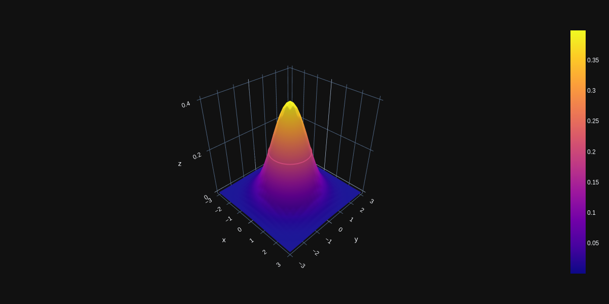
A Variational Auto-Encoder (VAE) interprets the input data, the latent representation of this input data and its conditional output as approximations to the standard normal distribution. The typical auto-encoder stores its representation in latent space as singular points (as explained above), whilst the VAE instead samples across probability distributions in latent space.
Approximate Standard Normal
The VAE learns an approximation to the posterior given some observed data, which is computed without needing the marginal of our above equation to be differentiable. This approximation is what constitutes the encoder, since given a data-point, it produces a distribution over the possible values of the latent variable z from which the data-point could be generated. From this viewpoint, \(p(x|z)\) is now our decoder, since it decodes, or translates the given latent variable into a distribution over possible corresponding values of x
Coming back to our cat-dog example, the encoder would code-ify dogs and cats images to standard normal distributions in latent space, whilst our decoder would attempt to reconstruct the original input images using only this code in latent space
Kullback–Leibler Divergence
An issue faced with the traditional, non-probabilistic auto-encoder lies in the overall distribution of the latent space. In other terms, the space within which a data-point is encoded is unbounded and the density of areas corresponding to different classes of data-points is far from uniform. This causes an issue for the decoder, where sampling from points too far from a very dense area results in 'predictions' that do not at all resemble the input data.
Using the KL-Divergence as a penalty term restricts the spread of classes in latent space. In addition to there now being a probability distribution about a point in latent space to be sample from (as opposed to single points), the KL-divergence is used to restrict or regularize the distribution of latent variables. This has the effect of reducing large gaps in latent space, since all encoded distributions are now coerced into resembling the standard-normal.
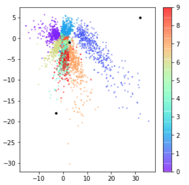
For example, the following are taken from the book Generative-Deep-Learning, where the first may represent what latent space may look like without the KL penalty term, and the second is after applying KL penalisation in order to regularise the codified latent space variables.
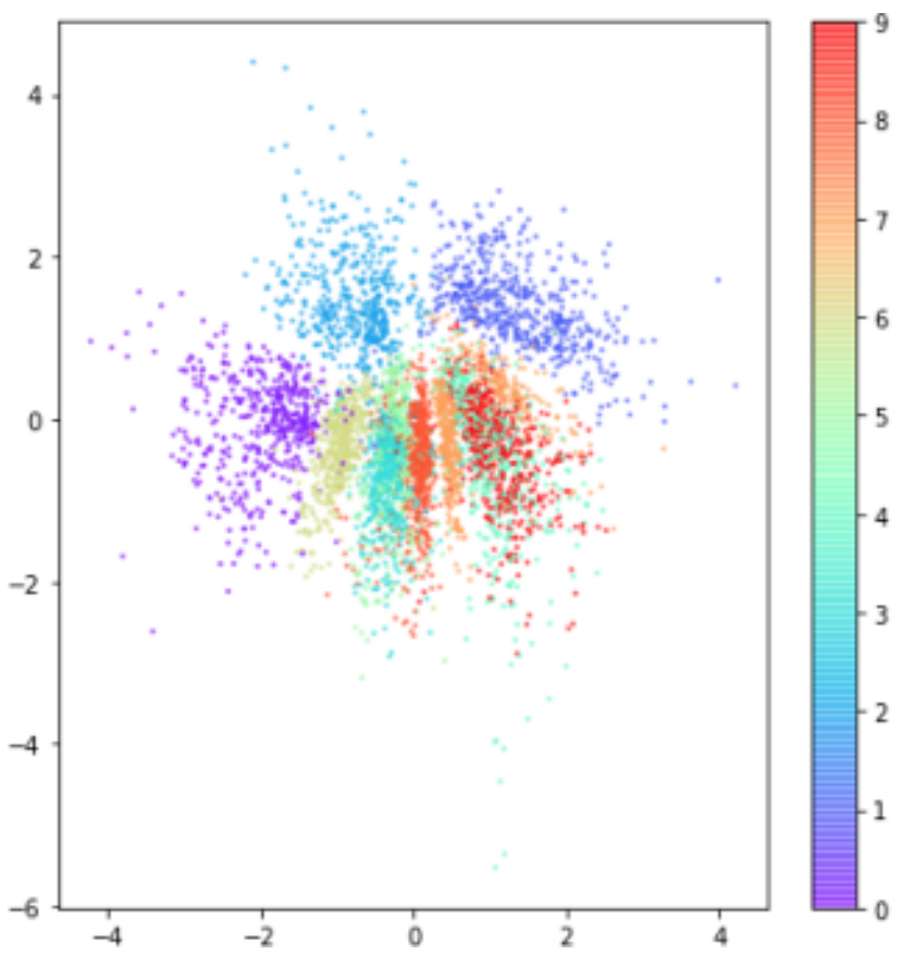
Additionally, sampling from an area just around the standard-normal results in parameters that highly resemble the distribution (this is what we want, in order to generate data close to our original, encoded data)
Summary
In brief, the VAE treats its input, latent variables and its output as probabilistic random variables. The encoder maps inputs to posterior distributions over latent space, and the deocder maps these latent representations into an approximation of the input data, with the main highlight being the KL-loss, which restricts these latent vectors to roughly unit Gaussian


